Marigold: Repurposing Diffusion-Based Image Generators for Monocular Depth Estimation

Bingxin Ke; Anton Obukhov; Shengyu Huang; Nando Metzger; Rodrigo Caye Daudt; Konrad Schindler

Marigold Repurposing Diffusion-Based Image Generators for Monocular Depth Estimation

We fine-tune the U-Net of Stable Diffusion v2 to denoise depth latents conditioned on the input image, leaving the VAE frozen. Trained on 74K synthetic samples in 2.5 GPU-days, Marigold estimates affine-invariant depth and transfers zero-shot to real indoor, outdoor and in-the-wild scenes.

Bingxin Ke·Anton Obukhov·Shengyu Huang·Nando Metzger·Rodrigo Caye Daudt·Konrad Schindler

ETH Zürich · CVPR 2024 (Oral)

Overview

A generative prior is all you need

Monocular depth is ill-posed from geometry alone: every pixel could be explained by a nearby small object or a distant large one. What resolves the ambiguity is prior knowledge of the visual world — object shapes, scene layouts, occlusion patterns. Stable Diffusion was trained on internet-scale images for precisely that knowledge, so we reuse it instead of learning priors from depth data. One image latent conditions the denoising process; only the U-Net changes; the frozen VAE carries both the image and the depth map.

The result is an affine-invariant depth estimator trained on 74K synthetic samples from Hypersim and Virtual KITTI — no real depth at any point — which transfers zero-shot to NYUv2, ScanNet, KITTI, ETH3D and DIODE and leads that comparison in most metrics.

74K synthetic training samples 18K iterations 2.5 days on one RTX 4090 0 real depth samples seen

Abstract

Monocular depth estimation is a fundamental computer vision task. Recovering 3D depth from a single image is geometrically ill-posed and requires scene understanding, so it is not surprising that the rise of deep learning has led to a breakthrough. The impressive progress of monocular depth estimators has mirrored the growth in model capacity, from relatively modest CNNs to large Transformer architectures. Still, monocular depth estimators tend to struggle when presented with images with unfamiliar content and layout, since their knowledge of the visual world is restricted by the data seen during training, and challenged by zero-shot generalization to new domains. This motivates us to explore whether the extensive priors captured in recent generative diffusion models can enable better, more generalizable depth estimation. We introduce Marigold, a method for affine-invariant monocular depth estimation that is derived from Stable Diffusion and retains its rich prior knowledge. To leverage it, we fine-tune the diffusion model on synthetic depth data and transfer it to real-world datasets in a zero-shot fashion. Our method sets a new state of the art in zero-shot depth estimation on multiple datasets, significantly outperforming existing methods. We hope that our findings spur further research on general-purpose diffusion-based depth estimation.

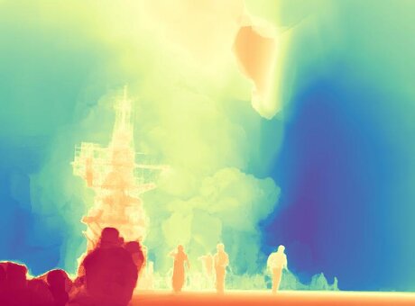
Colour encodes depth: red is near, blue is far. Everything below uses the same scale.

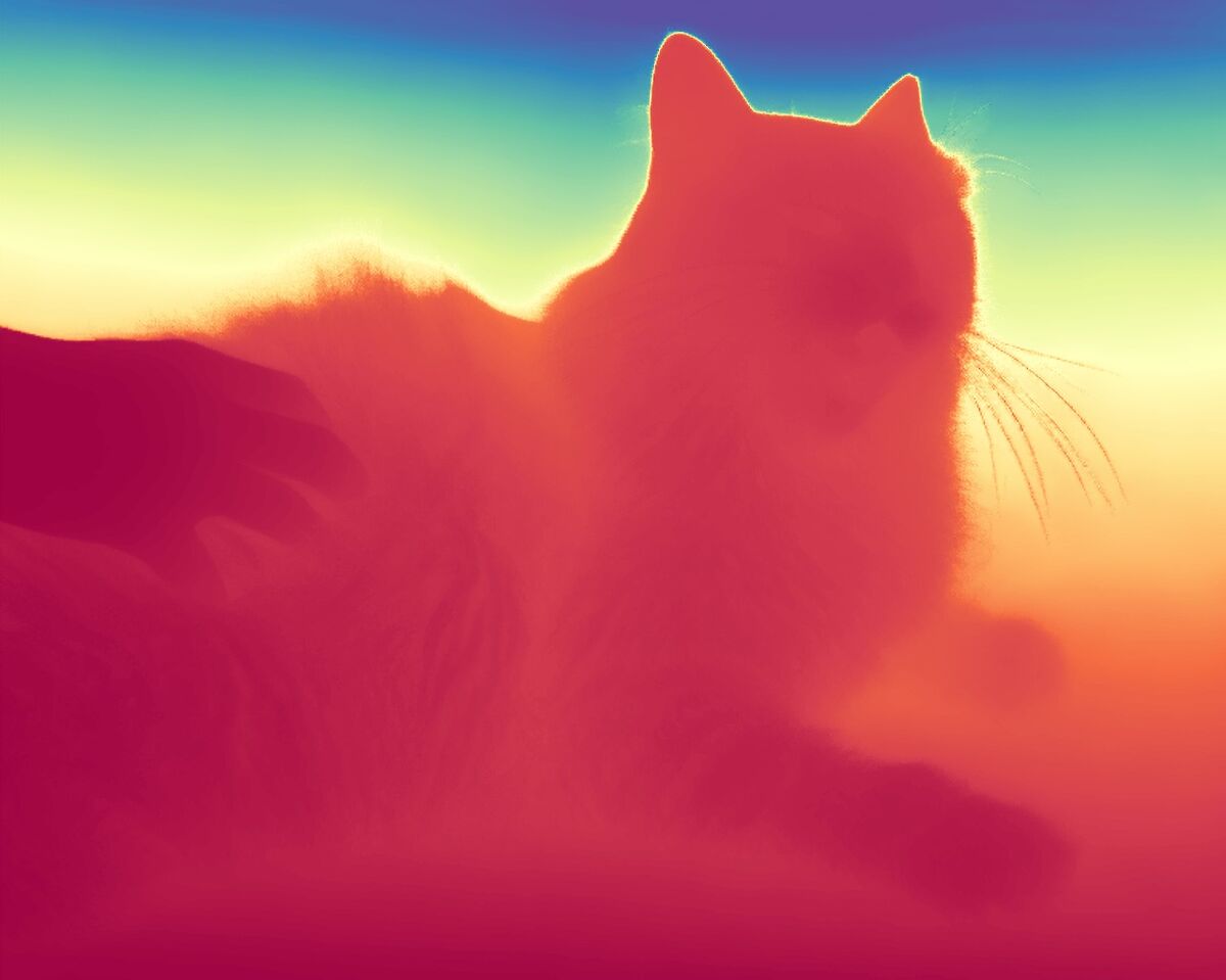Marigold depth map of a cat and a hand; fine detail around whiskers and fur — Hover the depth map to magnify. Whiskers, fur and the underside of the hand each carry their own depth; a smoother estimator loses them first.

Results

Drag to compare output with input

The child, the road surface, the trunks and the foliage behind them all sit at their own depth. Slide back and forth to check the two views against each other.

Marigold affine-invariant depth map of the same forest road, red near to blue far — Forest road, 3733×2800 input. Marigold keeps the trunks, the road and the canopy behind them apart; the colour scale is shared with every other comparison on this page.

Input photograph: a child running along a winding forest road — Forest road, 3733×2800 input. Marigold keeps the trunks, the road and the canopy behind them apart; the colour scale is shared with every other comparison on this page.

Fine detail

Where the difference shows

Single whiskers survive the depth map; DPT smears the whole head.

Full-resolution input↔depth comparisons with the released v1.1 checkpoint (DDIM trailing, 4 steps, ensemble of 5, processing resolution 768, output at native input size). The baseline is DPT-Large, whose affine-invariant disparity we show as 1 − normalised disparity so that both maps read on the same near-red / far-blue scale. Hover a map for the zoom lens.

How it works

Keep the latent space, train the denoiser

Marigold is Stable Diffusion v2 with its text conditioning replaced by an image. The U-Net denoises a depth latent $z^{(d)}$ , and the latent of the input image $z^{(x)}$ conditions every denoising step. Only the U-Net is trained; the VAE stays frozen, so the latent space in which the image prior lives stays intact.

Fine-tuning: the depth map is normalised to

[-1,1]

, replicated to three channels and encoded; image and depth latents are concatenated; the U-Net's first layer is widened to take both, its pretrained weights duplicated and halved so activation scale is preserved.

The fine-tuning figure as drawn in the paper

Fine-tuning protocol figure: frozen VAE encodes image and depth, U-Net trained with the diffusion objective

The protocol in numbers

Backbone: Stable Diffusion v2, v-objective
Trained parameters: U-Net only (VAE frozen)
Training data: 74K synthetic samples (Hypersim, Virtual KITTI)
Iterations: 18K, batch 32, 16 accumulation steps
Optimiser: Adam, lr 3·10⁻⁵
Training schedule: 1000 DDPM steps, annealed multi-resolution noise
Inference: 50 DDIM steps, 10 runs ensembled
Hardware: One RTX 4090, 2.5 days

What goes into the VAE

A depth map has no canonical units, and the VAE expects data in $[-1, 1]$ . We fix the range per image with the 2nd and 98th percentile of that map, which pins down an affine-invariant representation — everything later, evaluation included, is defined up to one scale and one shift.

\tilde{\mathbf{d}} \;=\; \left( \frac{\mathbf{d} - \mathbf{d}_{2\%}}{\mathbf{d}_{98\%} - \mathbf{d}_{2\%}} \;-\; 0.5 \right) \times 2

The only objective

Everything above reduces to the plain diffusion noise objective on the depth latent, with the image latent as the condition. No depth-specific loss, no extra heads, no change to the latent space.

\mathcal{L} \;=\; \mathbb{E}_{\mathbf{d}_0,\ \bm{\epsilon}\sim\mathcal{N}(0,I),\ t\sim\mathcal{U}(T)} \left\| \bm{\epsilon} - \bm{\epsilon}_\theta\!\left(\mathbf{z}^{(d)}_t, \mathbf{z}^{(x)}, t\right) \right\|_2^2

The schedule is annealed multi-resolution noise: it converges faster than Gaussian noise and makes predictions more consistent across runs, which is the property the next block exploits.

Test-time ensembling, playable

Each inference run starts from its own noise, so each returns the same scene on its own arbitrary scale and shift. We look for the frame in which the runs agree with one another — the pixel-wise median of the individually rescaled predictions, with a guard term $\mathcal{R} = |\min(\mathbf{m})| + |1 - \max(\mathbf{m})|$ that stops the whole thing collapsing to a flat map.

\min_{s_1..s_N,\, t_1..t_N}\ \sqrt{\tfrac{1}{b}\sum_{i<j}\|\hat{\mathbf{d}}_i s_i + t_i - \hat{\mathbf{d}}_j s_j - t_j\|_2^2}\ +\ \lambda\,\mathcal{R}

Runs

N

3 step 0/40

The 3 runs, each on its own frame

Before

AbsRel 0.0%

After

AbsRel 0.0%

Run disagreement: 0.000 → 0.000
Range guard R: 0.000
Objective: 0.000
AbsRel vs the scene: 0.0% → 0.0%

A toy, not the trained model: the runs are one simple depth field (a floor, three steps, two boxes) put through random scale, shift and noise, and the alignment is a few hand-written gradient steps — the same objective, run here on $N \leq 6$ maps. Set $N = 1$ to watch the alignment do nothing useful, then raise it and press Auto: the spread between runs shrinks, the boxes and the step edges come back, and AbsRel drops. On NYUv2 the same effect on the real model takes AbsRel down by about 8% from one run to ten, and about 9.5% from one run to twenty.

Where the test-time alignment comes from

Each of the $N$ runs returns its own depth map on its own arbitrary scale and shift. Before they can be medianed, they must be brought into a common frame. With no ground truth available, we ask for the frame in which the runs agree with each other: minimise the RMS distance between every pair of rescaled predictions, subject to a unit-range guard that stops the trivial all-zero solution.

This is related to the optimisation behind MiDaS-style scale-and-shift alignment, except that the reference here is the ensemble itself rather than a ground-truth map.

Benchmarks

Zero-shot on five real datasets

Marigold was trained on synthetic depth only and never saw a real depth sample. Compared with six zero-shot depth estimators it leads five of the ten metric columns outright and takes the best average rank. Numbers are percentages; lower AbsRel is better, higher δ1 is better.

Method	Training samples		NYUv2		KITTI		ETH3D		ScanNet		DIODE		Avg. rank
Method	real	synthetic	AbsRel↓	δ1↑	AbsRel↓	δ1↑	AbsRel↓	δ1↑	AbsRel↓	δ1↑	AbsRel↓	δ1↑	Avg. rank
DiverseDepth	320K	—	11.7	87.5	19.0	70.4	22.8	69.4	10.9	88.2	37.6	63.1	7.6
MiDaS	2M	—	11.1	88.5	23.6	63.0	18.4	75.2	12.1	84.6	33.2	71.5	7.3
LeReS	300K	54K	9.0	91.6	14.9	78.4	17.1	77.7	9.1	91.7	27.1	76.6	5.2
Omnidata	11.9M	310K	7.4	94.5	14.9	83.5	16.6	77.8	7.5	93.6	33.9	74.2	4.8
HDN	300K	—	6.9	94.8	11.5	86.7	12.1	83.3	8.0	93.9	24.6	78.0	3.2
DPT	1.2M	188K	9.8	90.3	10.0	90.1	7.8	94.6	8.2	93.4	18.2	75.8	3.9
Marigold (no ensemble)	—*	74K	6.0	95.9	10.5	90.4	7.1	95.1	6.9	94.5	31.0	77.2	2.5
Marigold (ensemble)			5.5	96.4	9.9	91.6	6.5	96.0	6.4	95.1	30.8	77.3	1.4

^* Image–text data was used to pretrain Stable Diffusion. Most baseline numbers follow Metric3D; for ScanNet the split differs there, so all baselines were re-run on ours. Evaluation aligns each prediction to the ground truth by least squares before computing AbsRel and δ1.

In the wild

Photographs the model was never trained on

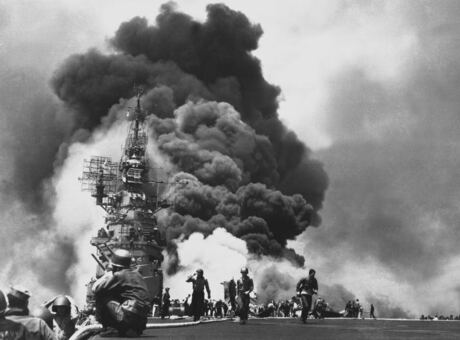
None of these scenes comes from a depth dataset: everyday photographs, drones, macro shots, museum rooms, archive film. Depth gives a scene a shape — the two clips below turn one prediction into a camera move and one into a wipe.

A 2.5D orbit: the photograph displaced by its predicted depth, so the pumpkins separate in space.

Input and depth wiped across each other: the whiskers arrive with the rest of the head instead of appearing later.

Depth maps. Hover a tile to see the input.

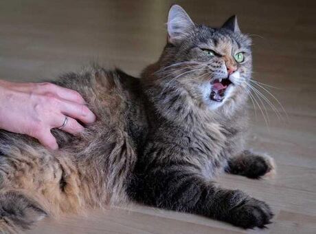
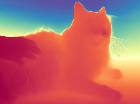
Cat
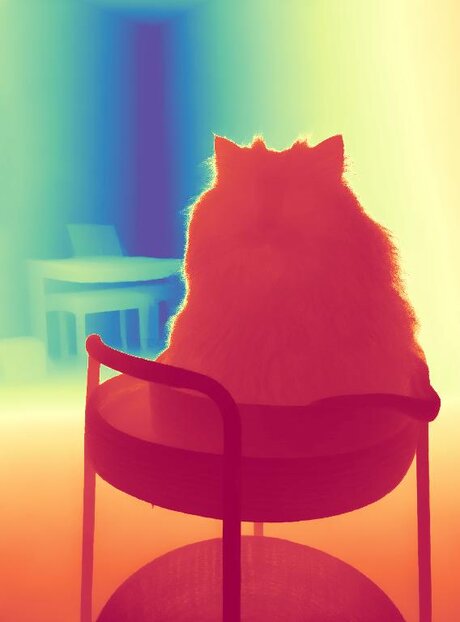
Cat in basket
Girl on swing
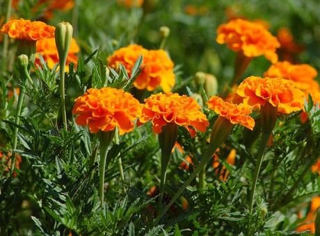
Marigold field
Marigolds close-up
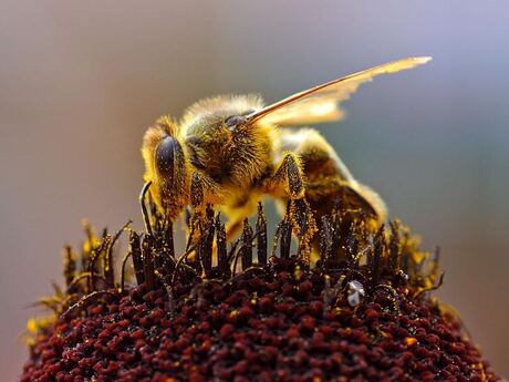
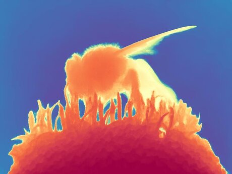
Bee on flower
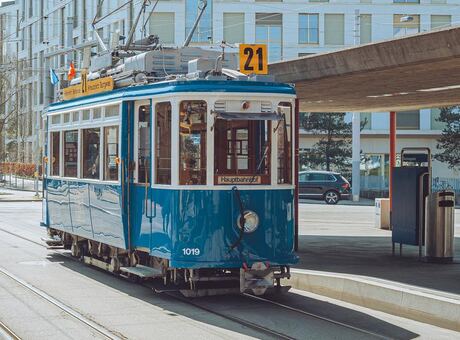
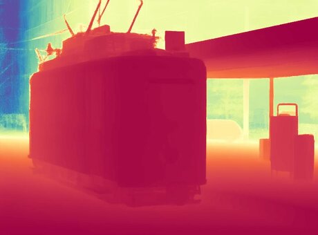
Zurich tram
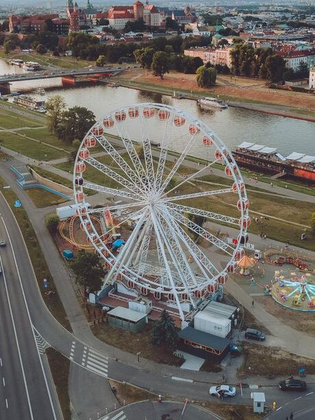
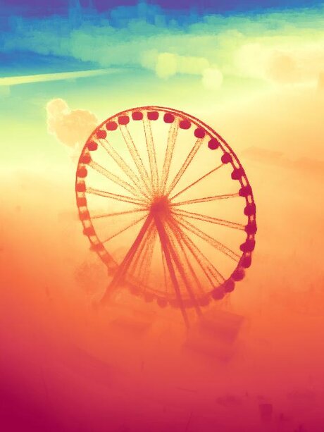
Ferris wheel
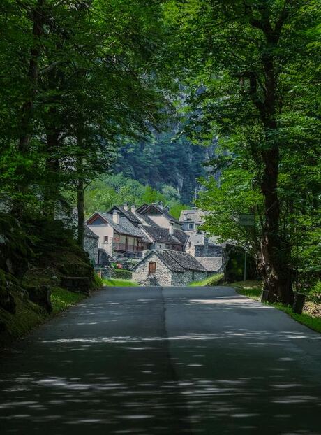
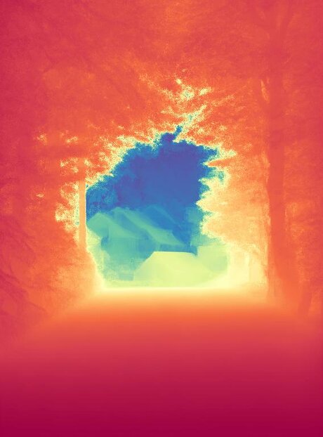
Forest road
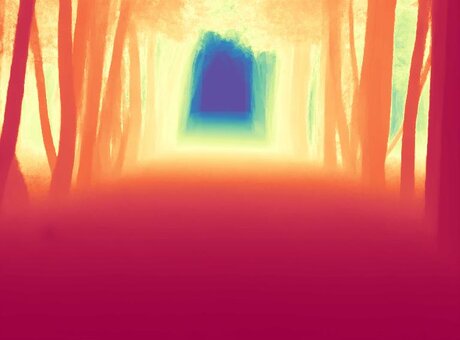
Tree-lined avenue
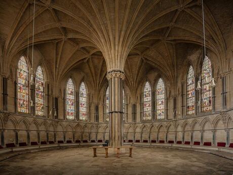
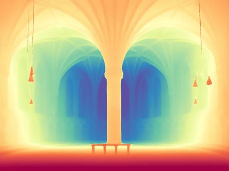
Chapter house
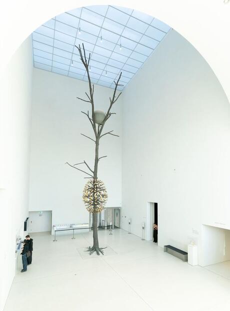
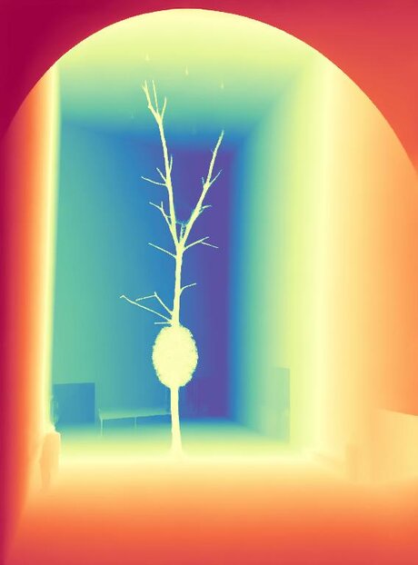
Gallery sculpture
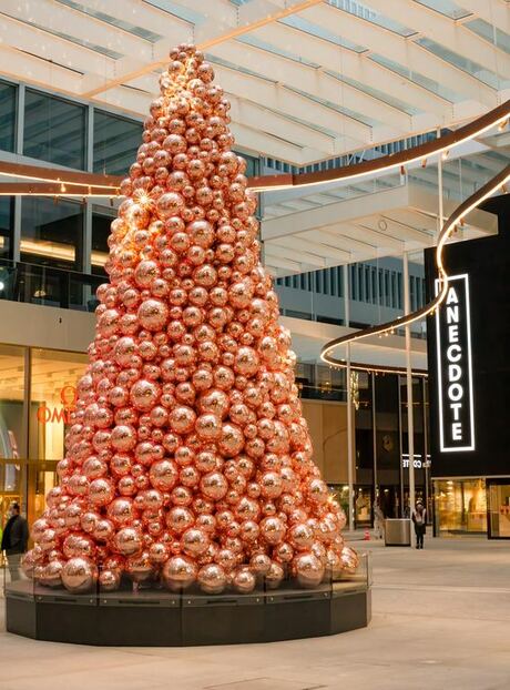
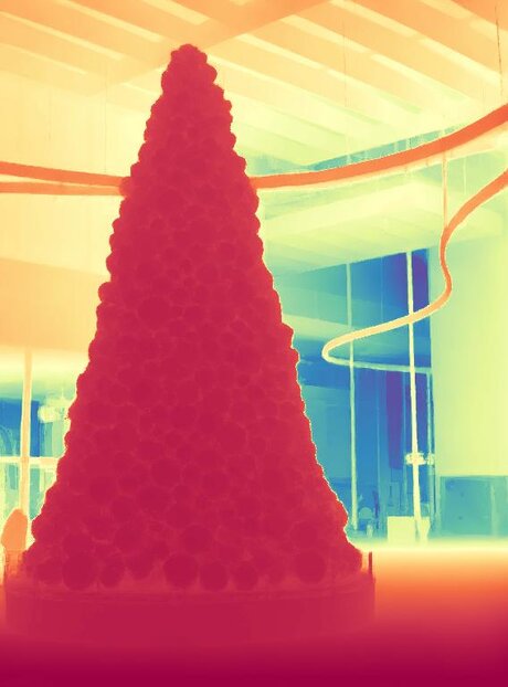
Bauble tree
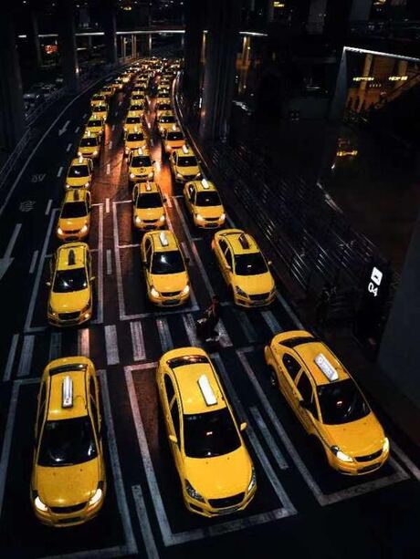
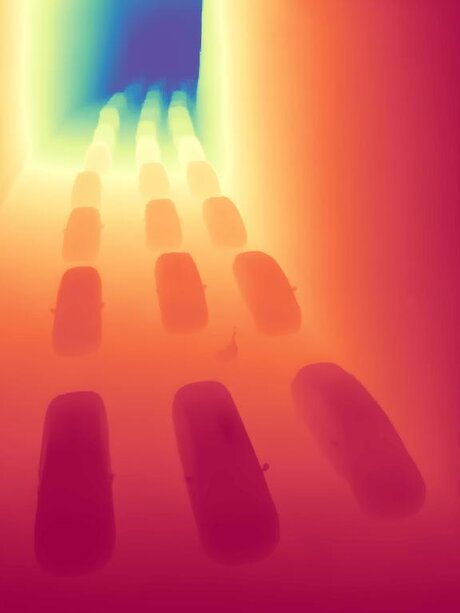
Taxis at night
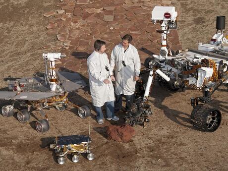
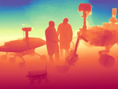
Mars rovers
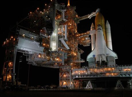
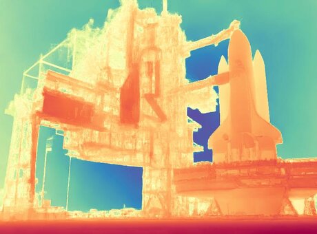
Shuttle at night
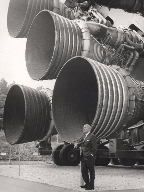
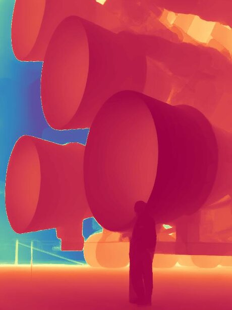
Saturn V, 1964
USS Bunker Hill, 1945

Citation

If it is useful, cite it

@inproceedings{ke2024marigold,
  title     = {Repurposing Diffusion-Based Image Generators for Monocular Depth Estimation},
  author    = {Ke, Bingxin and Obukhov, Anton and Huang, Shengyu and Metzger, Nando and Caye Daudt, Rodrigo and Schindler, Konrad},
  booktitle = {Proceedings of the IEEE/CVF Conference on Computer Vision and Pattern Recognition (CVPR)},
  year      = {2024}
}

CVPR 2024 (Oral) · code and weights are on GitHub and Hugging Face.